Hamming Distance and Hashing Functions

Description of the Problem

As yesterday, assume \((X,d)\) is a metric space of bitstrings of a fixed length together with the Hamming distance. Today, I am going to look at the distributions of numbers \(d(f(x),x)\) for \(x\in X\).

Implementation

As yesterday, I am going to use ironclad:

(require :ironclad)
NIL

and the same MD5 and SHA1 hashing functions:

(let ((hasher (ironclad:make-digest :md5)))
  (defun md5-digest (x)
    (coerce (ironclad:digest-sequence hasher x) 'list)))
MD5-DIGEST
(let ((hasher (ironclad:make-digest :sha1)))
    (defun sha1-digest (x)
       (coerce (ironclad:digest-sequence hasher x) 'list)))
SHA1-DIGEST

Since the space of bit strings of length 128 is large, I will use a Monte-Carlo method:

(defun random-vector (m)
   (coerce
      (loop repeat m collect (random 256))
      '(vector (unsigned-byte 8))))
RANDOM-VECTOR

And finally, the function that calculates the quantity I am interested in is

(defun hamming-distance (x y)
   (labels ((calc (x y &optional (acc 0))
               (cond
               ((< x y) (calc y x 0))
                 ((zerop x) acc)
                 (t (calc (ash x -1)
                          (ash y -1)
                          (if (equal (oddp x) (oddp y)) 
                             acc
                             (1+ acc)))))))
        (reduce #'+ (map 'list (lambda (i j) (calc i j)) x y))))
HAMMING-DISTANCE

Now, let me test this on a sample of size 40,000 on MD5:

(with-open-file (out "hamming2-data1.csv" :direction :output
                                          :if-exists :supersede
                                          :if-does-not-exist :create)
   (loop repeat 40000 do
       (let ((x (random-vector 16)))
          (format out "~4,9f~%" (/ (hamming-distance  (md5-digest x) x) 1.0)))))
NIL

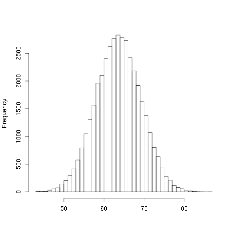
Here is a histogram of the data:

For the majority of the vectors, it is most likely that about 50% of the bits of the output will be different than the input.

Now, let me test this again on SHA1. Recall that since SHA1 digest produces 20 bytes, I am going to need random vectors of length 20:

(with-open-file (out "hamming2-data2.csv" :direction :output
                                          :if-exists :supersede
                                          :if-does-not-exist :create)
   (loop repeat 40000 do
       (let ((x (random-vector 20)))
          (format out "~4,9f~%" (/ (hamming-distance  (sha1-digest x) x) 1.0)))))
NIL

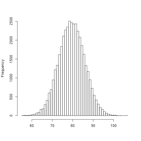
Here is a histogram of the data:

Again, about 50% of the bits are different between the input and output vectors.

An Analysis

I took the data from these experiments and normalized the values to the interval [0,1]. When I compared the distributions with the Kolmogorov-Smirnov test I see that

Two-sample Kolmogorov-Smirnov test

data:  normalize(as.matrix(X)) and normalize(as.matrix(Y))
D = 0.2524, p-value < 2.2e-16
alternative hypothesis: two-sided

which means that the distributions are different. Very interesting!