Graphs and Entropy
Description of the problem
Assume we have a directed graph with weighted edges. In other words,we have a triple \((V,E,w)\) such that
- \(V\) is a finite set
- \(E\) is a set of ordered pairs \((a,b)\) of elements from \(V\)
- \(w\colon E\to \mathbb{N}\) is a positive integer valued function
One can assume that weights can be arbitrary real numbers, but for thepurposes of today’s note, positive integer weights will do.
Today’s question is
How much randomness does a directed graph carry and how do wecalculate it?
Theory
For every graph \(G\), assume we have such a hypothetical measure\(\mu(G)\). We would like this measure to satisfy
Locality: The measure must be local, that is, one should be able to calculateit by looking at every vertex and only those vertices adjacent tothat vertex.
Additivity: If a graph contains two disjoint connected component, the totalmeasure should be the sum of the measures on each component.
Some Postulates
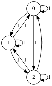
I would like to say that the complete graph on \(n\) vertices in whichevery edge has the same weight contains no information. For examplethe directed version of \(K_3\) (complete graph on 3 vertices) depicted below should not contain any information as every vertex is connected every other vertex in every way imaginable.
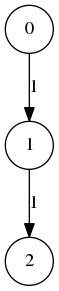
I would also like to say graphs in which there is no preference in the in the incoming edges contain no information either. Such as the line graphs \(A_n\) on \(n\) vertices,
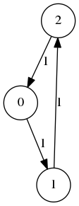
or cycle graphs \(C_n\) on \(n\) vertices:
A Candidate
The entropy is usually good measure to measure randomness in any probabilistic system. So, our first approximation is the randomness at a specific vertex. I’d like to measure the randomness in the incoming edges of a vertex. Assume \((V,E,w)\) is a weighted graph. I will write \(w_{ab}\) for the weight of an edge \(a\to b\). I will use the convention \[ w_{\cdot b} = \sum_{a\in V} w_{ab} \quad\text{ and }\quad w_{a\cdot} = \sum_{b\in V} w_{ab} \] In that case, I would like to say that \[ -\sum_{a\in V} \frac{w_{ab}}{w_{\cdot b}} \log_2\left(\frac{w_{ab}}{w_{\cdot b}}\right) \] measures the amount of information of the incoming edges of a vertex contains. Notice that this measure is scale invariant: if we replace \(w\) with \(\lambda w\) we get the same measure. However, this measure goes against our postulate that \(\mu(K_n)\) must be 0 since for every vertex in \(K_n\) we get \(\log_2(n)\). So, we will correct this measure by setting \[ E(b) = \log_2(\deg(b)) + \sum_{a\in V} \frac{w_{ab}}{w_{\cdot b}} \log_2\left(\frac{w_{ab}}{w_{\cdot b}}\right) \] which can be simplified to \[ E(b) = \log_2(\deg(b)) - \log_2(w_{\cdot b}) + \frac{1}{w_{\cdot b}}\sum_{a\in V} w_{ab}\log_2(w_{ab}) \] Then we define \[ \mu(G) = \sum_{b\in V} E(b) = \sum_{b\in V} \log_2(\deg(b)) - \sum_{b\in V}\log_2(w_{\cdot b}) + \sum_{a,b\in V} \frac{w_{ab}}{w_{\cdot b}}\log_2(w_{ab}) \] This measure is both local and additive. On top of that \(\mu(K_n)\), \(\mu(A_n)\) and \(\mu(C_n)\) are all zero.
The measure actually satisfies much more: if \((a,b)\in E\) is a bridge between two components \(G_1\) and \(G_2\),
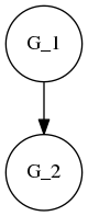
i.e. removing \((a,b)\) causes \(G\) to split into 2 connected components, then \(\mu(G) = \mu(G_1) + \mu(G_2)\) which is quite nice.
Implementation
I am going to represent each edge as a list of vertices \((a b)\) and weighted edges are going to be
a assoc list such as
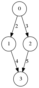
(defvar G
   `(((0 1) . 2)
     ((0 2) . 3)
     ((1 3) . 4)
     ((2 3) . 5)))
G
which will represent
I have been talking about map-reduce
and this is going to be good place to put it use:
(defun map-reduce (map red lis)
   (labels ((proc (x tail)
              (if (null x)
                 tail
                 (proc (cdr x)
                       (funcall red
                                (funcall map (car x))
                                tail)))))
       (proc lis nil)))
MAP-REDUCE
So, map-reduce takes a list lis maps over
it via map and then combines the results using
red. The following functions calculate the total flow (in
terms of weights) and the degree of a vertex.
(defun safe-add (x y) (+ (or x 0) (or y 0)))
SAFE-ADD

(defun flow (v G extract)
  (map-reduce (lambda (x)
                 (if (equal v (funcall extract x))
                    (cdr x)
                    0))
              #'safe-add
              G))
FLOW

(defun degree (v G extract)
  (map-reduce (lambda (x)
                 (if (equal v (funcall extract x))
                    1
                    0))
              #'safe-add
              G))
DEGREE
The passed argument extract extracts either the source
or the target of an edge depending on whether we want the outgoing flow,
incoming flow, outgoing degree or incoming degree.
Here comes the entropy function:
(defun entropy (v G extract)
  (labels ((saf (x) (if (zerop x) 1 x))
           (fn (x) (* x (log x 2))))
    (let ((deg (saf (degree v G extract)))
          (sum (saf (flow v G extract)))
          (int (map-reduce (lambda (x)
                             (if (equal v (funcall extract x))
                                 (fn (cdr x))
                                 0))
                           #'safe-add
                           G)))
      (+ (log deg 2) (- (log sum 2)) (/ int sum)))))
ENTROPY
And then we define the total entropy function as:
(defun total-entropy (G extract)
   (let ((vertices (remove-duplicates (map-reduce #'car #'append G))))
      (map-reduce (lambda (x) (entropy x G extract))
                  #'safe-add
                  vertices)))
TOTAL-ENTROPY
Some Tests
Let me define the following first before I do any tests:
(defun K (n)
   (loop for i from 0 below n append
      (loop for j from 0 below n collect
         (cons (list i j) 1))))
K

(defun A (n)
   (loop for i from 0 below (1- n) collect
      (cons (list i (1+ i)) 1)))
A

(defun C (n)
   (cons (cons (list (1- n) 0) 1) (A n)))
C
and calculate
(total-entropy (K (1+ (random 100))) #'cadar)
0.0f0
(total-entropy (A (1+ (random 100))) #'cadar)
0.0f0
(total-entropy (C (1+ (random 100))) #'caar)
0.0f0
How about the graph I defined earlier?
(total-entropy G #'cadar)
0.008924007f0
(total-entropy G #'caar)
0.029049516f0
So, by looking at these numbers, I wouldhttp://web.bahcesehir.edu.tr/atabey_kaygun/Blog/graphs-and-entropy.html say that the outgoing edges of \(G\) has more randomness than the incoming edges. And if I modify the graph into
(defvar H
   `(((0 1) . 1)
     ((0 2) . 2)
     ((1 3) . 1)
     ((2 3) . 2)))
H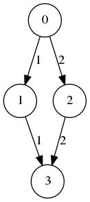
I will get the same numbers
(total-entropy H #'cadar)
0.0817042f0
(total-entropy H #'caar)
0.0817042f0
because the graph is symmetric.
An example
I had been looking at the Math PhD network. By calculating the graph entropy I’d like to see if there was any difference between randomness of the incoming and the outgoing edges.
So, first a function to load the data up. Data consists of 6 columns separated by tabs. Columns are the id of the math PhD degree coming from the Math Genealogy Project, advisor’s school (name and country) and PhD granting school’s name and country. Data is loaded as a assoc list based on an offset: if the offset is 0 then we construct the graph depending on the individual school, if the offset is 1 then we do a country based graph.
(defun load-data (name offset)
   (with-open-file (in name :direction :input)
      (let ((res nil)
            (pos-a (+ offset 1))
            (pos-b (+ offset 3)))
         (do ((line (read-line in nil) (read-line in nil)))
             ((null line) res)
           (let* ((local (cl-ppcre:split #\Tab line))
                  (a (elt local pos-a))
                  (b (elt local pos-b)))
              (if (assoc (list a b) res :test #'equal)
              (incf (cdr (assoc (list a b) res :test #'equal)))
              (push (cons (list a b) 1) res)))))))
LOAD-DATA
Now, let us see the entropy and their differences
I have two data sets: one data set consists of the math PhD’s awarded within the US, UK and Canada during the great recession (2007–2011), and the other math PhD’s awarded within the same period within Germany, Netherlands and Switzerland.
(defvar data1 (load-data "graphs-and-entropy-data1.csv" 1))
DATA1
(total-entropy data1 #'cadar)
937.71124f0
(total-entropy data1 #'caar)
919.27625f0
For the US, UK and Canadian Universities the measure of non-randomness was larger for the incoming edges as opposed to the outgoing edges. This means in this period, the universities show a larger preference of hiring professors in terms of their countries than granting PhD’s.
(defvar data2 (load-data "graphs-and-entropy-data2.csv" 1))
DATA2
(total-entropy data2 #'cadar)
556.59485f0
(total-entropy data2 #'caar)
619.4584f0
The situation is opposite for the universities in Germany, Netherlands and Switzerland.
When we repeat the same analysis for the university based graph, we see the same pattern.
(defvar data3 (load-data "graphs-and-entropy-data1.csv" 0))
DATA3

(total-entropy data3 #'cadar)
6245.294f0
(total-entropy data3 #'caar)
5241.133f0

(defvar data4 (load-data "graphs-and-entropy-data2.csv" 0))
DATA4

(total-entropy data4 #'cadar)
2096.72f0
(total-entropy data4 #'caar)
2122.4478f0
The discrepancy in the German, Netherlands and Switzerland case is much smaller, but it is far larger in the case of the UK, US and Canada case and in the opposite direction.