Uniform Sampling from Parametrized Submanifolds

Description of the problem

Assume we have a compact region \(\Omega\) defined in \(\mathbb{R}^n\) via an inequality of the form \(g(x_1,\ldots,x_n)\leq r\) where \(g(x_1,\ldots,x_n)\) is some nice function defined on \(\mathbb{R}^n\), For non-mathematicians out there, assume that the region I am talking about is bounded within a rectangular box, or that \(0\leq x_i\leq 1\) for \(i=1,\ldots,n\). Then we can sample points from \(\Omega\) uniformly by using an accept/reject algorithm:

1. we sample a sequence of numbers \((x_1,\ldots,x_n)\) where each \(x_i\) is a uniformly random number chosen in the unit interval,

2. if \(g(x_1,\ldots,x_n)\leq r\) accept it otherwise reject it.

This algorithm has a nice after-effect: if we record the accept rate then we can estimate the volume of the region \(\Omega\). The downside is that if the region is small then it is difficult to get points in \(\Omega\). And if the dimension of \(\Omega\) is strictly smaller than \(n\) (say you are trying to sample points on a curve embedded in the 3 dimensional space) then it is really really difficult (read almost impossible) to sample points using the accept/reject algorithm as the measure of \(\Omega\) within \(\mathbb{A}^n\) is 0.

Sampling from equidimensional regions

If the dimension of the region \(\Omega\) is the same as the ambient space then the accept/reject algorithm I described above works just fine. Here is an implementation is lisp

(defun sample (n test-fn)
   (let (test res)
      (do ()
          ((not (null test)) res)
        (setf res (loop repeat n collect (random 1.0d0)))
        (setf test (funcall test-fn res)))))


SAMPLE

We pass the dimension of the ambient space as well as a test function which describes our region. This function will return a uniformly random point from the region defined by the test function. Here is an example:

(defun sample-from-ellipse (a b)
   (sample 2 (lambda (v) 
                 (let ((x (elt v 0))
                       (y (elt v 1)))
                    (<= (+ (expt (/ x a) 2) (expt (/ y b) 2)) 1.0d0)))))

(sample-from-ellipse 0.1 9.0)


(0.011914196085003548d0 0.3981536986031673d0)

In the example above, we picked a uniformly random point within the ellipse \(100 x^2 + \frac{y^2}{81}\leq 1\).

Let me modify the function sample so that we see how many tries it took to get a sample point:

(defun sample (n test-fn)
   (let (test res)
      (do ((i 0 (1+ i)))
          ((not (null test)) (cons i res))
        (setf res (loop repeat n collect (random 1.0d0)))
        (setf test (funcall test-fn res)))))

(sample-from-ellipse 0.01 0.01)


(1225 0.002715773271653177d0 0.006181148622634192d0)

I was trying to sample a point from \(x^2 + y^2 \leq 10^{-4}\) the disk of radius \(0.01\), and it took some about 1000 tries before we hit a point within our region.

There is an alternative method: if our region \(\Omega\) is parametrized over the unit cube, that is, if there is a nice function (bijective and differentiable) \(f\colon \[0,1\]^n\to \Omega\) then we can sample points directly from \(\Omega\). The argument goes like this: calculate \(J(f)\) the Jacobian of \(f\) which is the determinant of the \(n\times n\)-matrix \(\left(\frac{\partial f_i}{\partial x_j}\right)\) where \(f_i\) is the i-th coordinate of the function \(f\). Consider the integral \[ F(a_1,\ldots,a_n) = \int_0^{a_1}\cdots \int_0^{a_n} J(f) dx_1\cdots dx_n \] Then \(F(a_1,\ldots,a_{i-1},x,a_{i+1},\ldots,a_n)\) must be a uniform random variable obeying the uniform distribution for every \(i=1,\ldots,n\) and \(a_1,\ldots,a_{i-1},a_{i+1},\ldots,a_n\in \[0,1\]\).

An equidimensional example

Let be demonstrate this with an example: consider the right triangle \(y\leq x\) with \(0\leq x\leq 1\). There is a parametrization of the region given by \[ f(x,y) = (x,yx) \] If we map the uniformly chosen points \((x,y)\) from the unit square directly into our right triangle we would see

(with-open-file (res "sampling-data1.csv" 
                     :direction :output 
                     :if-exists :supersede)
    (loop repeat 400 do
          (let ((x (random 1.0d0))
                (y (random 1.0d0)))
             (format res "~4,3F ~4,3F~%" x (* y x)))))


NIL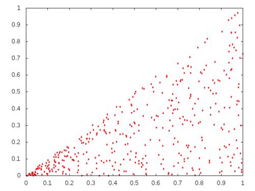

This is not what we want as we can see the condensation of points around the origin. The Jacobian of the parametrization is \[ \left\|\begin{matrix} 1 & y\\ 0 & x \end{matrix}\right\| = x \] then \[ F(a,b) = \int_0^a \int_0^b x dx dy = \frac{a^2 b}{2} \] must be a random number between 0 and ½. For \(a=1\), the expression \(\frac{b}{2}\) must produce uniformly random numbers in the interval \(\[0,½\]\). In other words, \(b\) is a uniformly random number between 0 and 1. For \(b=1\) we get \(\frac{a^2}{2}\) must be a uniformly random variable between 0 and ½ as \(a\) must be in \(\[0,1\]\). If \(x\) is a uniform random variable in the interval \(\[0,½\]\) then \[ \frac{a^2}{2} = x \quad \implies \quad a = \sqrt{2x} \] An implementation of the sampling a uniformly random point in the region we are interested in would look like

(defun sample-triangle ()
   (let ((x (sqrt (random 1.0d0)))
         (y (random 1.0d0)))
     (list x (* x y))))

(with-open-file (res "sampling-data2.csv" 
                     :direction :output 
                     :if-exists :supersede)
    (loop repeat 400 do
             (format res "~{~5,3F ~}~%" (sample-triangle))))


NIL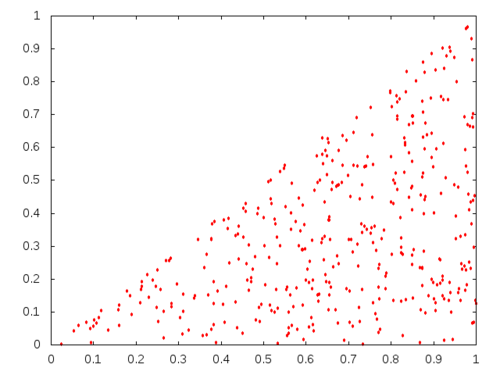

Notice that in the implementation I chose \(x\) in the interval \(\[0,1\]\) because if originally \(x\) is in \(\[0,½\]\) then \(2x\) would be in \(\[0,1\]\).

Another equidimensional example

This time, I will take my region to be the unit ball in the 3-dimensional space. I will use a modified version of the spherical coordinates: \[ x = \rho\cos(2\pi\theta)\sin(\pi\varphi), \quad y = \rho\sin(2\pi\theta)\sin(\pi\varphi), \quad z = \rho\cos(\pi\varphi) \] so that we can take \(\rho\in\[0,1\]\), \(\theta\in\[0,1\]\) and \(\varphi\in\[0,1\]\). The Jacobian is \[ J(f) = \left\|\begin{matrix} \cos(2\pi\theta)\sin(\pi\varphi) & \sin(2\pi\theta)\sin(\pi\varphi) & \sin(\pi\varphi) \\ -2\pi\rho\sin(2\pi\theta)\sin(\pi\varphi) & 2\pi\rho\cos(2\pi\theta)\sin(\pi\varphi) & 0 \\ \pi\rho\cos(2\pi\theta)\cos(\pi\varphi) & \pi\rho\cos(2\pi\theta)\cos(\pi\varphi) & -\pi\rho\sin(\pi\varphi) \end{matrix}\right\| = 2\pi^2\rho^2\sin(\pi\varphi) \] Then \[ F(a,b,c) = 2\pi^2\int_0^c\int_0^b\int_0^a \rho^2\sin(\pi\varphi) d\rho d\theta d\varphi = \frac{2\pi}{3} a^3 b (1-\cos(\pi c)) \] would generate random numbers between 0 and \(\frac{4\pi}{3}\), or equivalently \[ G(a,b,c) = \frac{3}{2\pi}\cdot 2\pi^2 \int_c^{½}\int_0^b\int_0^a \rho^2\sin(\pi\varphi) d\rho d\theta d\varphi = a^3 b \cos(\pi c) \] is a random number between 0 and 1 for every \(a\in \[0,1\]\), \(b\in\[0,1\]\) and \(c\in \[0,½\]\). Using a similar argument as the previous example, we get \[ a = \sqrt\[3\]{x}. \quad b = y,\quad c = \frac{\arccos(z)}{\pi} \] where \(x\) and \(y\) are uniformly random numbers in the unit interval, and \(z\) is a uniformly chosen number in \(\[-1,1\]\).

Here is an implementation

(defun sample-sphere ()
   (let* ((rho (expt (random 1.0d0) (/ 3.0d0)))
          (theta (random 1.0d0))
          (phi (/ (acos (- (random 2.0d0) 1.0d0)) pi))
          (x (* rho (cos (* 2 pi theta)) (sin (* pi phi))))
          (y (* rho (sin (* 2 pi theta)) (sin (* pi phi))))
          (z (* rho (cos (* pi phi)))))
     (list x y z)))

(with-open-file (res "sampling-data3.csv" 
                     :direction :output 
                     :if-exists :supersede)
    (loop repeat 1200 do
          (format res "~{~5,3F ~}~%" (sample-sphere))))


NIL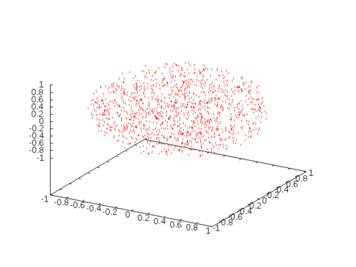

What happens if the region has strictly smaller dimension?

Say you’d like to sample points from a surface in the 3-dimensional space because you’d like to approximate it with a collection of triangles of approximately same size. How would you go about uniformly sample points? I will demonstrate this over the standard simplex \[ x+y+z=1 \quad\text{ with }\quad x,y,z\geq 0 \] in the 3-dimensional space. I will consider the following parametrization \[ (x,y,z) = f(a,b) = (ab,b-ab,1-b) \] where both \(s\) and \(t\) are numbers in the unit interval. The surface element of the parametrization is \[ \left\|\begin{matrix} \mathbf{i} & \mathbf{j} & \mathbf{k}\\ b & -b & 0 \\ a & 1-a & -1 \end{matrix}\right\| da\,db = \|b\mathbf{i} + b\mathbf{j} + b\mathbf{k}\| da\, db= b\sqrt{3}da\, db \] Then we get \[ F(u,v) = \int_0^u\int_0^v b\sqrt{3}da\,db = \frac{\sqrt{3}}{2} u^2 v \] From this equality we see that \(v\) must come from a uniformly random varible in the unit interval while \(u = \sqrt{x}\) where \(x\) is a uniformly random variable again in the unit interval.

(defun sample-simplex ()
   (let ((u (sqrt (random 1.0d0)))
         (v (random 1.0d0)))
      (list (* u v) (- u (* u v)) (- 1.0d0 u))))

(with-open-file (res "sampling-data4.csv" 
                     :direction :output 
                     :if-exists :supersede)
    (loop repeat 400 do
             (format res "~{~5,3F ~}~%" (sample-simplex))))


NIL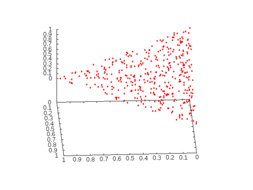

Then \[ \int_0^u\int_0^v J(f)d\theta\,d\phi\ = \int_0^u b\, d\phi\,\int_0^v (a + b\sin(v))d\theta = bu(av - b\cos(v) + b) \] assuming \(a \pi + 2b < 2 a \pi\) which is equivalent to \(2b < a \pi\) or \(\displaystyle\frac{2}{\pi} < \frac{a}{b}\). This equality allows us to conclude that \(u\) must be a uniform random variable and \(g(v) = av + b - b\cos(v)\) must be another uniform random variable. Now, we have an obvious problem of inverting the function \(g(v)\). If we choose \(a\) sufficiently larger than \(b\) then this function is close to \(h(v) = av\). For example for \(a=6.0\) and \(b=1.0\) we get the following graph for \(g(v)\)

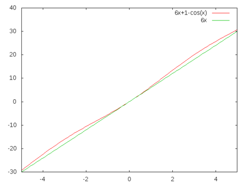
which isn’t much different than \(h(v)=6v\). This means, \(\theta\) although obeys a different probability distribution than the uniform distribution, is not that much different. So, using this simplification we get:

(defun sample-torus (a b)
   (let* ((theta (random (* 2.0d0 pi)))
          (phi   (random (* 2.0d0 pi)))
          (rho   (+ a (* b (cos theta))))
          (x     (* rho (sin phi)))
          (y     (* rho (cos phi)))
          (z     (* b (sin theta))))
      (list x y z)))

(with-open-file (res "sampling-data6.csv" 
                     :direction :output 
                     :if-exists :supersede)
    (loop repeat 1600 do
             (format res "~{~5,3F ~}~%" (sample-torus 6.0 1.0))))


NIL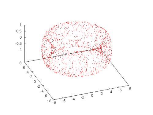

This is an approximation, of course. If we choose \(a\) and \(b\) closer, say \(a=1.2\) and \(b=1.0\) the situation will look much different (notice the condensation on the inner walls):

(with-open-file (res "sampling-data7.csv" 
                     :direction :output 
                     :if-exists :supersede)
    (loop repeat 1600 do
             (format res "~{~5,3F ~}~%" (sample-torus 1.2 1.0))))


NIL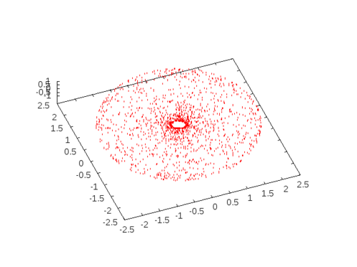

End note

Theoretically speaking, the result seems to be straight-forward: you must have a parametrized (over the unit cube) manifold embedded in \(\mathbb{R}^n\). Get the Jacobian, integrate it over any sub-cube and the resulting number must be a product of (as many as the dimension of the parametrized manifold) uniform random variables. If we are lucky, the result separates: that is the result is a product of separate functions one for each dimension. If we are extremely lucky, each of these functions is easily invertible [1] then we can apply the inverse functions to a sequence of uniformly random variables to obtain a distribution on the unit cube so that we get a uniformly distributed random points on our submanifold.

There is something missing in the argument above: I should really test that the points I get are truly uniformly random. That will be the subject matter of another post.