Simulated Annealing in Lisp

Today, I am going to look at a standard optimization algorithm called Simulated Annealing, and I will write an implementation in lisp. The algorithm is a heuristic one, and usually used to search for a near optimal solution within a fixed time period. It works by imitating a statistical mechanical process.

The algorithm

The Wikipedia page on Simulated Annealing is quite informative but for me the GNU Scientific Library’s page on the subject struck the perfect balance on being concise and informative. Here is my narrative on the algorithm. (All errors are mine, of course.)

The idea is that we randomly iterate our points using a stochastic process. The probability of jumping from one state to the randomly chosen next point depends on the ambient temperature. If the cost \(\phi(x_{i+1})\) in the next step is smaller than the cost \(\phi(x_i)\) at the current state then the probability of a jump is

\[ e^{ \frac{\phi(x_{i+1})-\phi(x_i)}{kT} } \]

Otherwise, the probability is set to 1.

Function SimulatedAnnealing
Input: cost, a cost function to be optimized
       init.pos, an initial point
       step, a function which iterates our approximation
       random, a uniform random number generator in [0,1] 
       init.temp, initial temperature
       k, a scaling parameter for temperature
       cooling, a function which gives us the temperature 
          in the next iteration
       min.temp, the temperature we stop
Output: pos, a near optimal minimum for the cost function
Initialize: temp <- init.temp
            pos <- init.pos
Begin
  While temp > temp.min do
     next <- step(pos, k, temp)
     if random() < exp( (cost(pos) - cost(next))/(k*temp) ) 
        pos <- next
     end
     temp <- cooling(temp, k)
  End
End

An implementation in lisp

Here is the code I wrote for the algorithm I described above:

(defun simulated-annealing (cost init step k init-temp cooling min-t &optional (trace nil))
     (labels ((obj (pos next temp)
                 (let ((a (funcall cost pos))
                       (b (funcall cost next)))
                    (exp (/ (- a b)
                            (* k temp)))))
              (iter (pos temp)
                 (let ((next (funcall step pos k temp)))
                    (if (> (obj pos next temp) (random 1.0d0))
                       next
                       pos))))
        (do* ((temp init-temp (funcall cooling temp))
              (pos init (iter pos temp))    
              (i 1 (1+ i)))
             ((< temp min-t) pos)
          (if (and trace (zerop (mod i 100)))
             (format t "~4d ~5,2f ~5,2f ~a~%" i temp (funcall cost pos) pos)))))

In my first example, I will try to minimize the function \(sin(exp(-x^2+x+1))\)

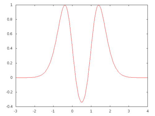
As one can see, the global minimum is hidden within a narrow valley. If the random iteration is incremental, that is if it uses Brownian motion, then it will get stuck in the large desert of local minima. It seems, if we know the approximate region where our near optimal solution lives, it is better to choose the next point completely random to avoid to get stuck in the local minima. So, I used a totally random iteration function which takes values in [-3,4] and does not use the current position. Initial position is set to 2.0, initial temperature is set to 100, minimal temperature is set to 0.001 and cooling schedule is multiplicative temp -> temp/1.01.

(simulated-annealing (lambda (x) (sin (exp (+ (* -1 x x) x 1))))
                      2.0d0
                      (lambda (x k temp) (- (random 7.0) 3.0))
                      1.0d-2
                      100
                      (lambda (temp) (/ temp 1.01))
                      1.0d-3)
0.51129866

Not bad.

Next up, the Himmelbrau function: \[ (x^2 + y - 11)^2 + (x + y^2 - 7)^2 \]

Here, the global minima are on the intersection of two parabolas \(y=11-x^2\) and \(x= 7 - y^2\). After some algebraic manipulation, you should see that the solution to the equation \[ y^4 - 14y^2 + y + 38 = 0 \] is what we need. There are 4 solutions:

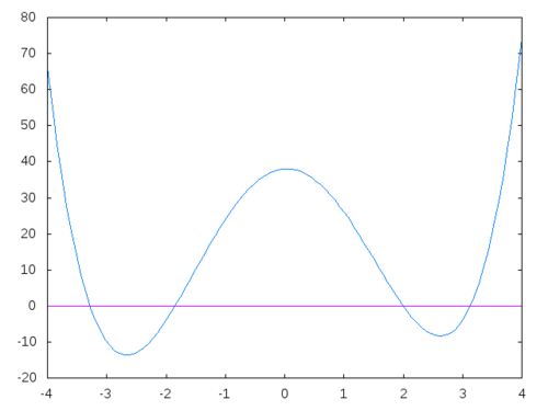
One of the possible solutions is y = -1.8481265269621736d0 and x = 3.584428340338734d0.

Here, I used a Brownian motion type iteration with the same cooling schedule function as above.

(simulated-annealing (lambda (v)
                        (let ((x (aref v 0))
                              (y (aref v 1)))
                           (+ (expt (+ -11.0d0 y (expt x 2)) 2)
                              (expt (+ -7.0d0 x (expt y 2)) 2))))
                     #(3.0 -2.0)
                     (lambda (v k temp)
                        (map 'vector (lambda (i) (+ i (- (random 0.2d0) 0.1d0)))  v))
                     1.0d-1
                     100.0
                     (lambda (x) (/ x 1.01))
                     1.0d-2)
#(3.5762820850832755d0 -1.8606108094272549d0)

Again, not too bad.

If I were to choose my next point in the iteration totally randomly, then if the algorithm to converge, it would converge to one of the possible 4 optimal points. With the Brownian motion type iteration, if we were to drop the initial point close to any of the other 3 possible solutions we would find the other points. Here let me find one other:

(simulated-annealing (lambda (v)
                        (let ((x (aref v 0))
                              (y (aref v 1)))
                           (+ (expt (+ -11.0d0 y (expt x 2)) 2)
                              (expt (+ -7.0d0 x (expt y 2)) 2))))
                     #(4.0 4.0)
                     (lambda (v k temp)
                        (map 'vector (lambda (i) (+ i (- (random 0.2d0) 0.1d0)))  v))
                     1.0d-1
                     100.0
                     (lambda (x) (/ x 1.01))
                     1.0d-2)
#(3.0015812084913107d0 2.008224658084634d0)

End note

I was thinking of implementing this in Julia too but J. M. White has already done it. As a matter of fact, I took idea of using SA to find the global minima for the Himmelbrau Function from him.