Collisions in random walks

Description of the problem

Imagine we have a directed graph in which each edge connecting a vertex $a$ to another vertex $b$ is labelled by the probability of jumping from $a$ to $b$. This precludes the condition that the sum of the labels of all outgoing edges is 1.

So, here is what I would like to consider today: if I have two particles moving between the states designated by the vertices of a directed graph according to the probabilities assigned to each edge, what is the probability of collision at step $n$?

An Unsatisfactory Solution

Assume we have $m$ possible states labelled by $1,\ldots,m$, and let $p_{ij}$ denote the probability of jumping from state $i$ to step $j$. If I form the transition matrix $P=(p_{ij})$ the entries of $P^n = (a_{ij})$ calculate the probability of jumping from state $i$ to state $j$ in $n$-steps. Then the probability of having a collision at step $n$ at a state $k$ is $a_{ik}a_{jk}$ if one particle starts at state $i$ and the other starts at $j$. If I would consider only the collision probability then \[ p_n(i,j) = \sum_{k=1}^m a_{ik} a_{jk} \] where, again, $(a_{ij})$ denote $P^n$ the entries of the $n$-th power of the transition matrix. A better way of writing the same equality goes through the observation that \[ p_n(i,j) = \sum_{k=1}^m a_{ik} a_{jk} = \sum_{k=1}^m a_{ik}a^t_{kj} \] where we use $(a^t_{ij})$ to denote the entries of the transpose $(P^t)^n$. In other words $p_n(i,j)$ is the $(i,j)$-th entry in the matrix $P^n (P^t)^n$. If the situation calls for checking existence of a collision regardless of where each particle starts then we must add all probabilities. Thus the total probability $p_n$ of a collision at step $n$ is the sum of all entries of the matrix $P^n (P^t)^n$ divided by $m^2$: \[ p_n = \frac{1}{m^2}\sum_{i,j,k} a_{ik}a_{ik} \] Division by $m^2$ happens because I assume all initial positions are assumed to be equally likely.

In most cases, $P^n$ stabilizes as $n$ goes to $\infty$, and therefore the probability $p_n$ also stabilizes. As $P^n$ stabilizes, the rows of the stabilized matrix become the 1-eigen vector of $P$. If that vector is $ < u_1,,u_m> $ then the stable collision probability is $\sum_{i=1}^m u_i^2$. This phenomenon will occur below in the examples I will use.

A More Suitable Solution

The solution I gave above checks if we have a solution at step $n$, and does not care if we have a collision before the step $n$. If the setup requires that we stop in the event of a collision then I must modify the solution.

We start with a different problem first: assume we have two subsets of vertices $A$ and $B$ in $V$, and let us try to find the probability of jumping from the combined state $A$ to the combined state $B$. Recall that $p_{ij}$ is a conditional probability: the probability of jumping to state $j$ given that we are at state $i$. So, the conditional probability of jumping to state $B$ from state $A$ is \[ \frac{\sum_{i\in A}\sum_{j\in B} p(i)p_{ij}}{\sum_{i\in A} p(i)} \] where $p(i)$ stands for the proability of being at state $i$. If we assume that $p(i)=\frac{1}{m}$, that is, every state is equally likely, then \[ p_{AB} = \frac{\frac{1}{m}\sum_{j\in B}\sum_{i\in A} p_{ij}}{\frac{\|A\|}{m}} = \frac{1}{\|A\|}\sum_{i\in A}\sum_{j\in B} p_{ij} \] Now, observe that for a pair of particles, the product $p_{i_1j_1}p_{i_2j_2}$ measures the conditional probability of the pair jumping respectively to the states $i_2$ and $j_2$ from states $i_1$ and $j_1$. Then the conditional probability of jumping into a collision state from a collision state is \[ P(C\|C) = \frac{1}{m}\sum_{i_1=j_1}\sum_{i_2=j_2} p_{i_1i_2} p_{j_1j_2} = \frac{1}{m}\sum_{i,j} p_{ij}^2 \] From a non-collision state to a collision state

For notational simplicity, I will use $\Psi$ for $P(C\|NC)$ and $\Phi$ for $P(C\|C)$. Then the probability of jumping from a collision state to a non-collision state \[ P(NC\|C) = 1 - P(C\|C) = 1 - \Phi\] and finally from a non-collision state to a collision state \[ P(NC\|NC) = 1 - P(C\|NC) = 1 - \Psi \] Let $q_n$ denote the probability of seeing our first collision at step $n$. Then \[ q_n = \left(1-\frac{1}{m}\right) (1 - \Psi)^{n-1}\Psi \] Then the expected number of steps before we see our first collision is \[ \sum_{n\geq 1} n q_n = \left(1-\frac{1}{m}\right)\Psi \sum_{n\geq 1} n (1 - \Psi)^{n-1} \] The last terms should be familiar from your calculus classes: it is the derivative of the power series $\sum_{n=0}x^n = \frac{1}{1-x}$ evaluated at $x=1-\Psi$. This is $\frac{1}{\Psi^2}$, and therefore, the expected number of steps for seeing a first collision is \[ \left(1-\frac{1}{m}\right)\frac{1}{\Psi} \]

A Small Variation

What if I would like to calculate the expected number of steps between two collisions? That is, I am going to have two particles starting at the same position and then wait until they collide again. What is the expected number of steps until that happens? I will use $h_n$ to denote probability of that happening at step $n$. This is the conditional probability of seeing the first collision at step $n$ given that we start with a collision state. For $n=1$ we have $h_1 = P(C\|C) = \Phi$. And for $n\geq 2$ \[ h_n = (1 - \Phi )( 1 - \Psi )^{n-2} \Psi \] Then the expected number of steps between two collision becomes \[ E = (1-\Phi)\Psi\sum_{n\geq 2} (n-1) (1-\Psi)^{n-2} = (1-\Phi)\Psi\sum_{n\geq 1} n (1-\Psi)^{n-1} \] Again the series is the derivative of the function $\frac{1}{1-x}$ evaluated at $1-\Psi$. Then \[ E = \frac{(1-\Phi)}{\Psi} \]

Implementation

 import numpy as np
 import math

 def see(P,n):
     if n < 0:
        res = 0
     else:
        res = (P**n)*(P.transpose())**n
     return res.flatten().sum()/P.size

 def c2c(P):
     return np.matrix([x**2 for x in P.flat]).sum()/math.sqrt(P.size)

 def nc2c(P):
     m = math.sqrt(P.size)
     return 1/(m-1)*( (P*P.transpose()).sum()/m - c2c(P) )

 def collision(P,n):
     if n < 0:
        res = 0
     elif n == 0:
        res = 1/math.sqrt(P.size)
     else:
        psi = nc2c(P) 
        res = (1.0 - 1.0/math.sqrt(P.size))*( 1.0 - psi )**(n-1)*psi
     return res 

 def total(P,N):
     res = 0
     if N > -1:
        for i in range(N):
            res += collision(P,i)
     return res

 def firstCollision(P):
     psi = nc2c(P)
     m = math.sqrt(P.size)
     return (1.0 - 1.0/m)*(1.0/psi) 

 def betweenCollisions(P):
     psi = nc2c(P)
     phi = c2c(P)
     m = math.sqrt(P.size)
     return (1.0-phi)/psi

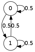
Now, let me consider a very simple setup

The corresponding transition matrix is

 P = np.matrix([[0.5, 0.5],
               [0.5, 0.5]])

and the corresponding collision probabilities are

n = 0	n = 1	n = 2	n = 3	n = 4	n = 5	n = 6	n = 7	n = 8	n = 9	n = 10
0.5	0.5	0.5	0.5	0.5	0.5	0.5	0.5	0.5	0.5	0.5
0.5	0.25	0.125	0.0625	0.0313	0.0156	0.0078	0.0039	0.002	0.001	0.0005

The first row lists the probabilities of seeing a collision at step $n$ regardless of seeing previous collisions. The second row lists the probabilities of seeing our first collisions at step $n$. The probability of seeing a collision within 10 steps is 0.999. The expected number of steps before we see our first collision is 1.0 and the expected number of steps between two collisions is 1.0.

Now, let me work with a setup in which collisions are impossible except at step $n=0$.

 P = np.matrix([[1.0, 0.0],
                [0.0, 1.0]])

and the corresponding collision probabilities are

n = 0	n = 1	n = 2	n = 3	n = 4	n = 5	n = 6	n = 7	n = 8	n = 9	n = 10
0.5	0.5	0.5	0.5	0.5	0.5	0.5	0.5	0.5	0.5	0.5
0.5	0.0	0.0	0.0	0.0	0.0	0.0	0.0	0.0	0.0	0.0

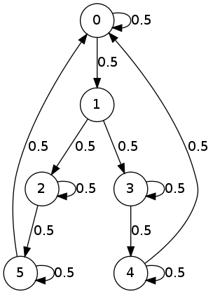
Now, let me consider the graph and the probabilities I gave at the beginning.

 P = np.matrix([[0.5, 0.5, 0.0, 0.0, 0.0, 0.0],
               [0.0, 0.0, 0.5, 0.5, 0.0, 0.0],
               [0.0, 0.0, 0.5, 0.0, 0.0, 0.5],
               [0.0, 0.0, 0.0, 0.5, 0.5, 0.0],
               [0.5, 0.0, 0.0, 0.0, 0.5, 0.0],
               [0.5, 0.0, 0.0, 0.0, 0.0, 0.5]])

Let me calculate the probabilities of a collision from $n=0$ to $n=20$.

n = 0	n = 1	n = 2	n = 3	n = 4	n = 5	n = 6	n = 7	n = 8	n = 9	n = 10	n = 11	n = 12	n = 13	n = 14	n = 15	n = 16	n = 17	n = 18	n = 19	n = 20
0.1667	0.1806	0.1875	0.1927	0.189	0.1841	0.1818	0.1821	0.1833	0.1842	0.1842	0.1839	0.1836	0.1835	0.1836	0.1837	0.1837	0.1837	0.1837	0.1837	0.1837
0.1667	0.0972	0.0859	0.0759	0.067	0.0592	0.0523	0.0462	0.0408	0.036	0.0318	0.0281	0.0248	0.0219	0.0194	0.0171	0.0151	0.0134	0.0118	0.0104	0.0092

In this situation seeing a collision at step $n$ stabilizes as expected, at 0.1837 after about 15 steps. On the other hand, the probability of seeing our first collision at step $n$ decreases to zero, as it should. And the total probability of seeing a collision during the first 20 steps is about 0.9211 . The expected number of steps before we see our first collision is 7.1429 and the expected number of steps between two collisions is 4.2857.